Introduction

The aim of this study is to determine the characteristics of ice flow in Austwick and to assess whether erratics are important to our understanding of how the Earth’s surface appeared thousands of years ago. By the end of this report, I aim to reach a conclusion regarding the origin of the Norber Erratics and their current positions, with a further examination of how they were transported to their current location.

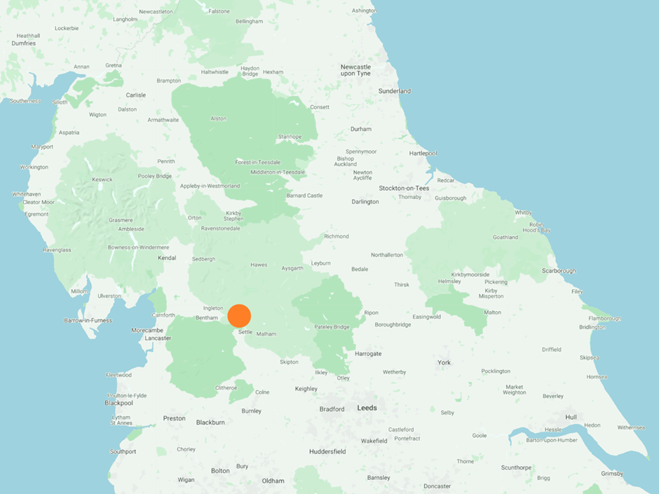
Figure 1 – Map showcasing the location of Austwick. Picture from Paul Beal

Austwick, shown in Figure 1, is a small town in the Yorkshire Dales National Park with a population of approximately 480 in 2021 (VisitSettle, 2023). The town is known geographically for its proximity to the Norber Erratics, large boulders plucked from the bedrock and deposited by glaciers some 17,000 years ago during the last glacial maximum (Emery, 2023). Figure 2 shows one such erratic from the Norber Erratics.

Erratics are very important because they help us understand the Earth during the ice ages thousands of years ago. To elaborate, erratics are, most of the time, made up of a different rock type than that of the bedrock they sit on in the present day. This means that the rock that makes up the erratic is of a different lithology. This requires immense force, which is why scientists know it had to be ice that was the main transporter rather than a river. By looking at the lithology of the erratic and that of the surrounding land, you can start to make accurate assumptions as to where the erratic may have been plucked from, which in turn gives an idea as to the direction of the flow of ice.

Figure 2 – An erratic that constitutes one of many just like this from the Norber Erratics.

Method

When gathering data, it is imperative to use multiple pieces of equipment to measure the different characteristics of the boulders and the surrounding landscape. The measurements to take are as follows:

Roundness: Roundness helps identify the location at which the boulders were transported, whether inside, on top, or at the base of the glacier. These measurements are to be made using a visual scale, so the final judgement will rest with the individual. Therefore, when performing this measurement, it is best to have the same person perform each step to ensure consistency. Because the roundness is measured by eye, this will likely be the least accurate data available.

Boulder shape: Use a tape measure to measure the long, intermediate, and short axes of the boulder, rounding the measurement up to the nearest 0.5cm. This can pose problems when measuring larger boulders, as the person conducting the measurements may have to climb them to take some measurements, and the boulders can be very slippery.

Boulder Fabric: Measuring the spatial and geometric configuration of the boulders using a compass clinometer. This data is crucial for determining the direction of ice flow during the last glacial maximum. When conducting these measurements, pick a point that represents the general ciliation of the boulder, as some areas that have been eroded may be showing a clinician that does not represent the majority of the boulder.

Spatial distribution of boulders: using a GPS at each of the measured boulders to plot the GPS coordinates onto a grid to showcase the distribution of each one. The distribution of boulders provides a clear visual representation of the study area and the number of samples, enabling the creation of a specialised distribution graph that aids data analysis.

Boulder Volume: Using the dimensions gathered from ‘boulder shape’, put those figures into the equation for an octahedral, which is 1/3 x root(2) x (H x W x D).

Having the same person gather and record the different measurements should make the results much more reliable.

Results

The major areas of study on the boulders were: roundness, boulder shape, boulder fabric, spatial distribution, and boulder volume. In total, during this study, 57 samples were taken at the start of the Norber Erratics field. These samples were taken from boulders that ranged greatly in size in order to give the highest range of possible data points.

Roundness

Judging by the roundness reading, I would assume that the samples were mainly transported on top of the glacier, as most of the samples are either angular or slightly angular (see Figure 3). However, I have some samples that are ’rounded’; therefore, it is reasonable to infer that they were transported at the edge of the glacier, as the boulders scraping against the valley side rounded themselves slightly. It would not be accurate to say that they were transported by water, as their angles remain too well-defined. Furthermore, on multiple occasions, when looking at the samples, you could see striations in the transported rocks, which would reinforce the idea that some scraped along the bedrock.

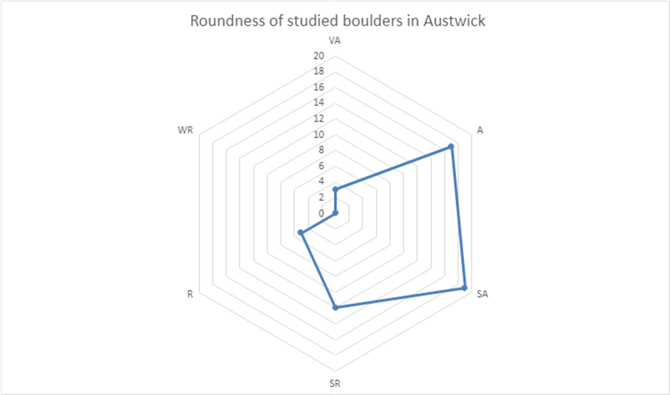
Figure 3 – A graph showcasing the roundness of the studied boulders.

Boulder shape

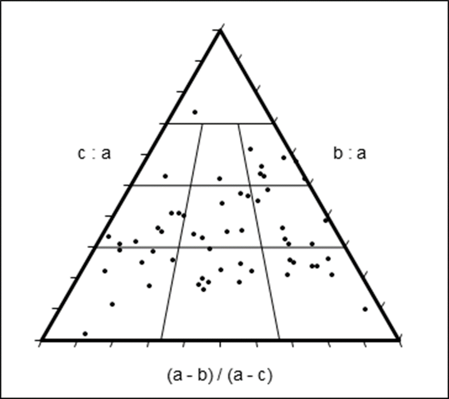
Figure 4 – A diagram showcasing all the particle shapes of the studied boulders.

The overall shape of the diagram in Figure 4 shows a variety of data points. However, most of them are congregated in the central region of the diagram. This indicates that most boulders range from platy to highly elongated, whereas very few, if any, are blocky, demonstrating that erosional forces have sculpted them. This is also backed by the data in Figure 5, which showcases what Figure 4 is showing clearly.

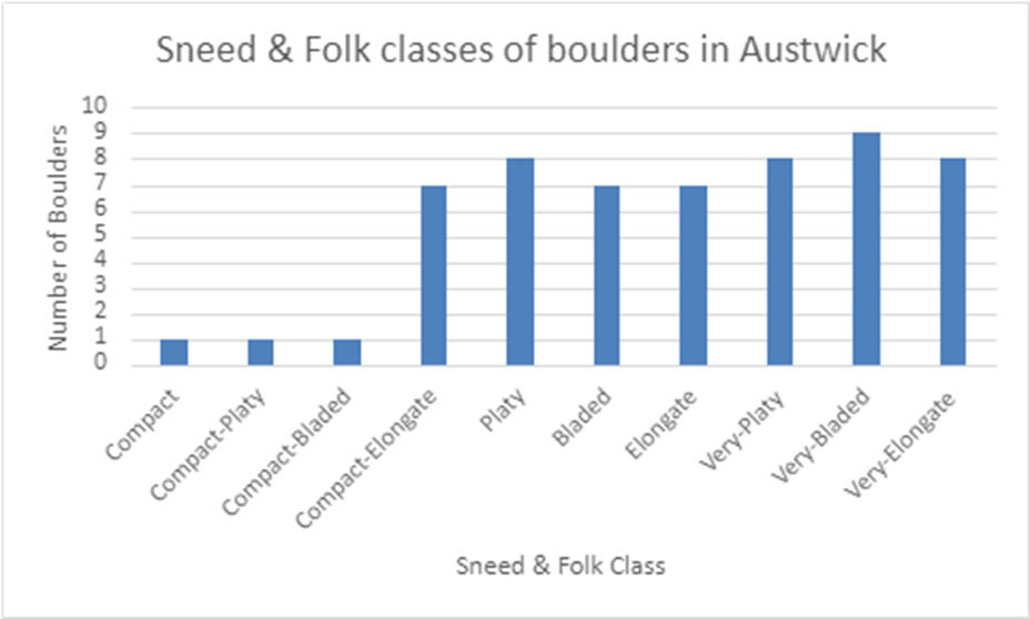
Figure 5 – A bar chart showing the boulder classification from the samples taken in Austwick.

The transport pathway corroborates the conclusion I drew from the roundness data. As the data suggest, the samples were predominantly intermediate between angular and rounded, further indicating that the primary mode of transport was supraglacial, as I concluded earlier.  

I believe that most of the samples that I took, Figure 6, were from newly eroded sandstone, as they were close to meeting the criteria outlined in Figure 7 but fell short because of their RA value, which is the percentage of boulders that are angular or very angular (Benn & Ballantyne, 1993). Indicating that the samples had not had enough time to become round enough to qualify for the given categories.  

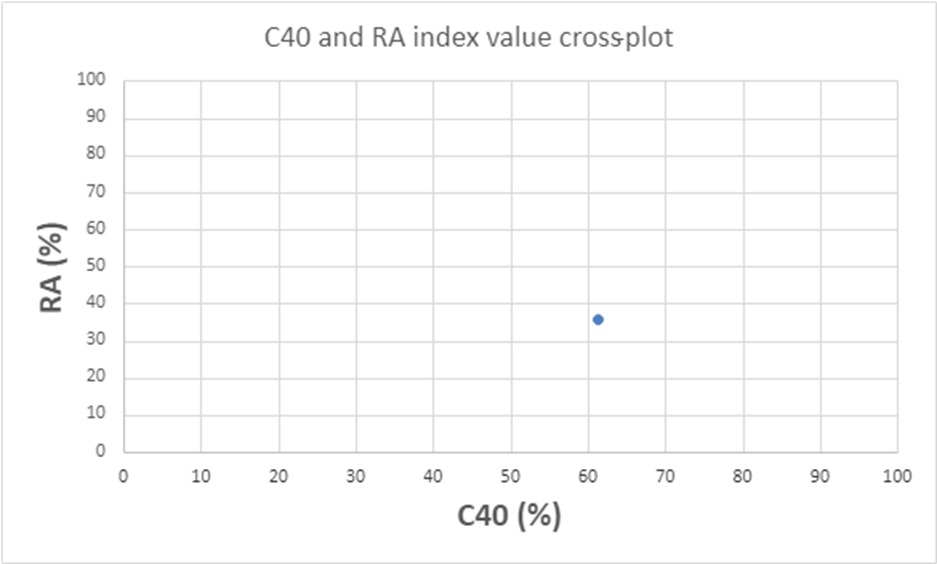
Figure 6 – A cross plot putting RA against C40

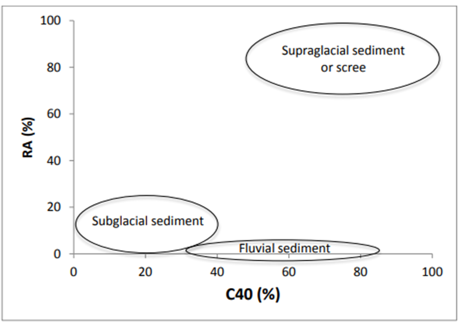
Figure 7 – A graph showcasing what the results in Figure 6 say about the sampled boulders

Boulder fabric

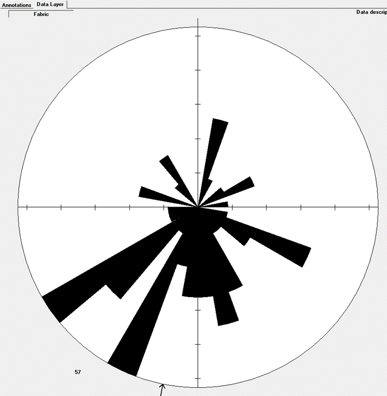
Figure 8 – A rose diagram showing the orientation of the sampled boulders

My data in Figure 8 display a strong orientation. Between 170 and about 240 degrees is the predominant orientation. This ice flowed in this general direction. This fits with the general consensus that the ice sheet came from Scandinavia and down south, meaning the ice came from a south-westerly direction, which is showcased in Figure 8. This data also aligns with those in Figure 5, which show that over one-third (38.6%) of the sampled boulders were either compact-elongate, elongated, or very elongated.

Boulder volume

Taking one of the boulder measurements as an example, it had an a-axis of 314cm, a b-axis of 337cm, and a c-axis of75cm, respectively. As it is not a cube, it must be put into the octahedral volume equation, which is 1/3 x root(2) x (H x W x D). This gives you an end octahedral volume of 4m³, making sure to divide by one million to convert cm³. After doing this for all 57 samples, we obtained an overall volume of 130 m³. This ranged from samples with an octahedral volume of 0.2 m³ to 39 m³.

Spatial distribution of boulders

The distribution of the samples in Figure 9 is clustered, indicating a high concentration of Erratics in the sampled area. This indicates that these boulders were randomly dropped in place rather than placed by humans.

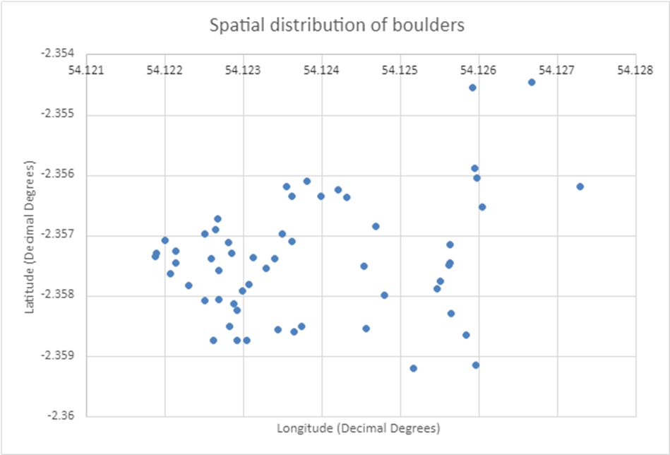
Figure 9 – A spatial distribution graph of all 57 boulder samples

The origins

The Norber Erratics have a lithology of Greywacke, which is very different from the limestone bed on which they now rest. When looking at the underlying lithology of the region, the point marked by Crummack Dale, highlighted in red in Figure 10, stands out as having a section layer of the Gerywacke on the south side of the hill. This would align with the data I obtained on the boulder’s fabric and alignment, indicating that it was transported approximately 1 mile to its current location. This indicates that the ice flowed very uniformly towards Austwick.  

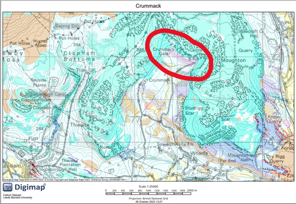
Figure 10 – A map showing the lithology of the rock in and around Austwick

Discussion

There have been several studies to determine where they originated. A study by Huddersfield University concluded that Crummack Dale, the Austwick Anticline, and the Kilnsey Formation were the primary sources of the Greywacke, with other locations mentioned in the conclusion but given less emphasis. (Parry, 2007)

The results of this study indicate that ice sheets during the last glacial maximum originated in the north and flowed south, transporting large volumes of moraine. This follows a similar pattern to that observed by a study conducted by the University of Liverpool of the lower Ribble Valley, which demonstrated the existence of moraine just south of Austwick. Therefore, signalling these erratic’s were deposited near the snout of the glacier (RICHARD C. CHIVERRELL, 2016).

It is also worth noting that the region where the Norber Erratics are found is highly exposed to the elements; therefore, data such as roundness, which affects the C40 and RA index values as well as shape, have been altered by processes unrelated to glaciers.

It is difficult to analyse the distribution of the samples as they are all situated close together; therefore, to get a better understanding of the region’s glacial past, it would be best to increase the area of study and the number of samples taken. Further data could be from the wider Ribble Valley to help work out the direction of the flow of ice before it got to Austwick. Finally, the lay of the land proved challenging, with very steep-sided cliffs that made it practically impossible to take measurements in certain areas, which is why there are large gaps in the graph. If I got extra data, I would make sure I had adequate footwear and equipment to get more results.

Using the spatial distribution to draw a conclusion on the maximum extent of the British-Irish ice sheet would not provide concrete evidence, as for one, we have found out that the source of these erratic’s are only a few miles away. Furthermore, their roundness and shape do not constitute a boulder that has undergone much glacial erosion. Finally, we cannot determine whether the boulder was transported atop the glacier and subsequently deposited where it is now, as temperatures rose. This would have been around 11,300 years ago (Emery, 2020).

Some of the results were not as clear as I expected, for example, though boulder fabric shows a strong correlation between southeastern and western alignments. I was expecting a much stronger association, as though the current one still supports the idea of a north-south flow. It opens up new questions as to why some erratic’s are aligned towards the southeast while others are from the southwest.

Conclusion

To conclude, the study found that the boulders just north of Austwick, Norber, were not boulders but erratics that are approximately 11,000 years old. This was proven by the level of erosion that the Erratic had gone through, including the striations that were present on some.

Furthermore, the different lithology of the erratic proves that it cannot have originated from its current location, as the lithology does not match. I have further concluded that the glaciers that traversed the region originated in the north and flowed south, transporting boulders with them. This was proven by the orientation of the erratics, which showed a strong correlation to a south-easterly and South-westerly orientation. I also deduced that these boulders were transported down on top of the glacier (supraglacial) as they were not rounded enough to be interpreted as boulders that came into contact with water and did not possess many, if any, striations that would be indicative of contact with bedrock at the base of the ice mass.

This information will help people understand how Earth’s landscape looked over 11,000 years ago and may provide scientists with insights into what to expect as the world’s glaciers retreat rapidly due to global warming.

References

Benn, D. I. & Ballantyne, C. K., 1993. The description and representation of practical shape. Earth Surface Processes and Landforms, VII(18), pp. 665-672.

Emery, A., 2020. The LGM British-Irish Ice Sheet: an introduction. [Online]
Available at: https://www.antarcticglaciers.org/glacial-geology/british-irish-ice-sheet/last-glacial-maximum/the-british-irish-ice-sheet-an-introduction/#:~:text=All%20of%20Scotland%20and%20Ireland,by%2011%2C300%20years%20ago3.

Emery, A., 2023. Glacial Erratics. [Online]
Available at: https://www.antarcticglaciers.org/glacial-geology/glacial-landforms/glacial-depositional-landforms/glacial-erratics/
[Accessed 26 October 2023].

Parry, B., 2007. THE PROVENANCE OF THE NORBER ERRATICS, AND THE FORMATION OF POST-DEVENSIANDEGLACIATION PEDESTAL ROCKS WITH CARBONIFEROUS LIMESTONE PEDESTALS IN ENGLAND, IRELAND AND WALES., Huddersfield: University of Huddersfield.

RICHARD C. CHIVERRELL, M. J. B. a. G. S. T., 2016. Morphological and sedimentary responses to ice mass interaction during the last deglaciation. Journal of Quaternary Science, 3(31), pp. 265-280.

VisitSettle, 2023. Austwick. [Online]
Available at: https://www.visitsettle.co.uk/austwick.html
[Accessed 27 November 2023].